================
Overview of the challenge
Food delivery companies connects consumers with their favorite resturants through machine-learning-backed service. Once the order arrives late, the convinence due to delivery now becomes frustration.

To ensure that the prediction of delivery time closely reflects the actual delivery time, information from the three sides involved - the store, the dashers’ capacity, and the consumer’s order - all needs to be taken into consideration.
Conceptually, the estimated delivery duration after the customer placing an order can be divided into these components (it’s not necessarily a chain of events since some can be done in paralell):
- The time that a store takes to receive an order from DoorDash
- The time for a store to repare for an order
- Assigning the order to the right dasher
- The dasher travels to the store
- The dasher picks up order and goes to the destination
- The time of dashing trying to find the specific location of delivery after getting off delivery vehicle
Overview of the approach
- New features like “Weekday or Weekend” and “Day or Night” for are created for each delivery job based on exisiting date-and-time data to extract information useful for time prediction. These features makes the model more accurate since it captures the clustered effects like stores’ kitchens being busier during weekends than weekdays, and delivery jobs with daylight being eaiser and faster than they are after dark.
- Other potential new features (e.g. average parking time at a specific lcoation) that could further improve the model are raised and discussed below.
- The potential models of time prediction are evaluated both by the mean of abosolute errors with the actual delivery time and a categorical metric that better fulfills the business goal. Specifically, the categorical metric separates delivery predictions based on their over/underestimation of the actual duration. And there are 6 ordinal slots that ranks each delivery prediction from “Very late - over 10 min” to “Very early - over 10 min”. When interpreting and evaluating the model performance, the lateness (underestimating the delivery) are penalized more than early estimations (overestimating the delivery time), and very late/early deliveries should be viewed as stronger signals of call for model improvement than being slightly late/early.
Models used
- A linear regression model was created first. The model does well in keeping the overall late delivery within 15%, and the very-late (over 5 minutes) deliveries is around 6.9%. But the RMSE score is high - 1672.92. Note: Overall lateness is defined as the proportion of late delivery, which ranges from very late (over 10 min) to about on time (late within 5 min).
- A mixed effect model with the store_id as random effects (meaning that we can later take these irrelevant clustering effect out to make our estimation of the meaningful variables more accurate). The mixed effect model outperformed the linear regression on both the RMSE (1627.13) and the lateness (very late: 6.3%, overall lateness: 14.1%).
- A XGBoost model also performs well with a low “very late” (6.8%) delivery and slightly higher overal lateness (14.9%) than the mixed effect model . Although the cross validation RMSE of the XGBoost model (1478.721) is much lower.
- As those the XGBoost and the mixed effect model are very different, averaging predictions is likely to improve the predictions. In the prediction for submission, I averaged the prediction between the XGBoost model and the mixed effect model, with higher weight given to the XGBoost model.
Introduction and potential NEW features to add
The dataset provides 16 important aspects of a typical delivery. But there are much more could influence the time cost of a duration:
Below I raise and discuss 5 potential new features that could improve the model performance, if collected
1. Community/Zipcode
The location of the destinations alters the delivery time. Destinations in suburb areas have easier access and parking than locations in urbdan enviroment, where tall buildings and stricter security is more common. Further, during weekdays the parking at urban area might be harder than suburb community, and this flunctuation in parking time throughout the week is not captured by the existing estimated point-to-point duration.
2. Condo vs. Home
This feature provides a more detailed account of the environments of the destination than the Community feature above. Condos are in buildings (with stairs and/or security entrance), which means longer time is needed between getting off the delivery car and arriving at the customer’s door.
3. Weather
Although the estimated point-to-point delivery by other models captures the weather of that day, the impact of weather on the first and the last mile of the delivery might still impacted by the weather. For instance, potential delay in delivery caused by heavy precipitation can be taken into calculation with this new feature.
4. Vehicle of delivery
Whether the vehicle of delivery has four wheels or two wheels significantly impact how big of an order a dasher can take. This would make the number of available dashers for a certain order more accurate, which enhances the capacity prediction.
5. Average parking time at a specific location
As more and more datapoints accumulate, the average time to park at a specific location would be more accurate. This feature could siginificantly improve the model fit.
Further reading: A relevant paper I found online Order Fulfillment Cycle Time Estimation for On-Demand Food Delivery by Zhu et al.
Loading and Exploring Existing Data
##Loading libraries required and reading the data into R
cat("\f")
rm(list = ls())
library(readr)
library(knitr)
library(ggplot2)
library(plyr)
library(dplyr)
library(corrplot)
library(caret)
library(gridExtra)
library(scales)
library(Rmisc)
library(ggrepel)
library(psych)
library(xgboost)
library(skimr)
library(lme4)
library(merTools)
library(mice)
library(lubridate)


library(apa)
devtools::install_github("crsh/citr")
library(citr)
library(papaja)
library(MOTE)
library(tidyverse)
library(kableExtra)
Below, I am reading the csv’s as dataframes into R.
train_raw = read_csv("/Users/guoxinqieve/Applications/OneDrive - UC San Diego/DD_takeHomeExercise/historical_data.csv")
test_raw = read_csv("/Users/guoxinqieve/Applications/OneDrive - UC San Diego/DD_takeHomeExercise/predict_data.csv")
#Pre-processing - data exploration, recoding, and cleaning
# overview of the variables
glimpse(train_raw)
## Rows: 197,428
## Columns: 16
## $ market_id                                    <dbl> 1, 2, 3, 3, 3, 3, 3, 3, 2…
## $ created_at                                   <dttm> 2015-02-06 22:24:17, 201…
## $ actual_delivery_time                         <dttm> 2015-02-06 23:27:16, 201…
## $ store_id                                     <dbl> 1845, 5477, 5477, 5477, 5…
## $ store_primary_category                       <chr> "american", "mexican", NA…
## $ order_protocol                               <dbl> 1, 2, 1, 1, 1, 1, 1, 1, 3…
## $ total_items                                  <dbl> 4, 1, 1, 6, 3, 3, 2, 4, 4…
## $ subtotal                                     <dbl> 3441, 1900, 1900, 6900, 3…
## $ num_distinct_items                           <dbl> 4, 1, 1, 5, 3, 3, 2, 4, 3…
## $ min_item_price                               <dbl> 557, 1400, 1900, 600, 110…
## $ max_item_price                               <dbl> 1239, 1400, 1900, 1800, 1…
## $ total_onshift_dashers                        <dbl> 33, 1, 1, 1, 6, 2, 10, 7,…
## $ total_busy_dashers                           <dbl> 14, 2, 0, 1, 6, 2, 9, 8, …
## $ total_outstanding_orders                     <dbl> 21, 2, 0, 2, 9, 2, 9, 7, …
## $ estimated_order_place_duration               <dbl> 446, 446, 446, 446, 446, …
## $ estimated_store_to_consumer_driving_duration <dbl> 861, 690, 690, 289, 650, …
glimpse(test_raw)
## Rows: 54,778
## Columns: 17
## $ market_id                                    <dbl> 3, 3, 4, 3, 1, 1, 1, 1, 1…
## $ created_at                                   <dttm> 2015-02-25 02:22:30, 201…
## $ store_id                                     <dbl> 5477, 5477, 5477, 5477, 2…
## $ store_primary_category                       <chr> NA, NA, "thai", NA, "ital…
## $ order_protocol                               <dbl> 1, 1, 1, 1, 1, 1, 1, 1, 1…
## $ total_items                                  <dbl> 5, 5, 4, 1, 2, 3, 2, 1, 1…
## $ subtotal                                     <dbl> 7500, 7100, 4500, 1700, 3…
## $ num_distinct_items                           <dbl> 4, 4, 2, 1, 2, 3, 2, 1, 1…
## $ min_item_price                               <dbl> 800, 800, 750, 1400, 1525…
## $ max_item_price                               <dbl> 1800, 1500, 1500, 1400, 1…
## $ total_onshift_dashers                        <dbl> 4, 4, 9, 3, 4, 5, 11, 11,…
## $ total_busy_dashers                           <dbl> 4, 1, 7, 3, 4, 3, 11, 10,…
## $ total_outstanding_orders                     <dbl> 4, 1, 6, 3, 4, 3, 16, 10,…
## $ estimated_order_place_duration               <dbl> 446, 446, 446, 446, 446, …
## $ estimated_store_to_consumer_driving_duration <dbl> 670, 446, 504, 687, 528, …
## $ delivery_id                                  <dbl> 194096, 236895, 190868, 1…
## $ platform                                     <chr> "android", "other", "andr…
# recoding to make the variables type match the description
# (some numeric columns should be categorical)
train = train_raw %>%
    mutate(market_id = as.character(market_id), store_id = as.character(store_id),
        store_primary_category = as.character(store_primary_category),
        order_protocol = as.character(order_protocol))

test = test_raw %>%
    mutate(market_id = as.character(market_id), store_id = as.character(store_id),
        store_primary_category = as.character(store_primary_category),
        order_protocol = as.character(order_protocol))
summary(train$created_at) # created_at No NAs, but has a weird minimal: '2014-10-19 05:24:15' this should be excluded
##                       Min.                    1st Qu.
## "2014-10-19 05:24:15.0000" "2015-01-29 02:32:42.0000"
##                     Median                       Mean
## "2015-02-05 03:29:09.5000" "2015-02-04 22:00:09.5379"
##                    3rd Qu.                       Max.
## "2015-02-12 01:39:18.5000" "2015-02-18 06:00:44.0000"
train$created_at[year(train$created_at) == 2014] = NA  # now the earliest created_at is in year 2015

summary(train$actual_delivery_time)  # actual_delivery_time has 7 NAs, other than that looks normal
##                       Min.                    1st Qu.
## "2015-01-21 15:58:11.0000" "2015-01-29 03:22:29.0000"
##                     Median                       Mean
## "2015-02-05 04:40:41.0000" "2015-02-04 22:48:23.3489"
##                    3rd Qu.                       Max.
## "2015-02-12 02:25:26.0000" "2015-02-19 22:45:31.0000"
##                       NA's
##                        "7"
# looking at the distribution of the type of cuisines
table(train$store_primary_category)  # some categories are much more popular than the others.
##
##            afghan           african           alcohol alcohol-plus-food
##               119                10              1850                 1
##          american         argentine             asian          barbecue
##             19399                72              2449              2722
##           belgian         brazilian         breakfast           british
##                 2               310              5425               133
##        bubble-tea            burger           burmese              cafe
##               519             10958               821              2229
##             cajun         caribbean          catering            cheese
##               316               253              1633                24
##           chinese         chocolate      comfort-food convenience-store
##              9421                 1                28               348
##           dessert           dim-sum         ethiopian          european
##              8773              1112               134                22
##              fast          filipino            french         gastropub
##              7372               260               575               184
##            german       gluten-free             greek          hawaiian
##                68                62              3326              1499
##            indian        indonesian             irish           italian
##              7314                 2                55              7179
##          japanese            korean            kosher    latin-american
##              9196              1813                51               520
##          lebanese         malaysian     mediterranean           mexican
##                 9               102              5512             17099
##    middle-eastern          moroccan          nepalese             other
##              1501                25               299              3988
##         pakistani             pasta           persian          peruvian
##               139               633               607               254
##             pizza           russian             salad          sandwich
##             17321                19              3745             10060
##           seafood       singaporean          smoothie              soup
##              2730                33              1659                74
##          southern           spanish             steak             sushi
##               156                37              1092              2187
##             tapas              thai           turkish             vegan
##               146              7225               237               279
##        vegetarian        vietnamese
##               845              6095
# looking at the distribution of the means of how stores
# accpet order
table(train$order_protocol)  # order_protocol has a lot of NAs, ranges from 1 to 7, are distinct, some are much more popular than others
##
##     1     2     3     4     5     6     7
## 54725 24052 53199 19354 44290   794    19
summary(train$order_protocol)
##    Length     Class      Mode
##    197428 character character
# looking at the number of items in total
summary(train$total_items)  # ranges form 1 to more than 411, No NAs
##    Min. 1st Qu.  Median    Mean 3rd Qu.    Max.
##   1.000   2.000   3.000   3.196   4.000 411.000

# looking at the subtotal of the order
summary(train$subtotal)  # the min is zero, the median is 2200, highest 27100
##    Min. 1st Qu.  Median    Mean 3rd Qu.    Max.
##       0    1400    2200    2682    3395   27100
# looking at the # of unique items of the order
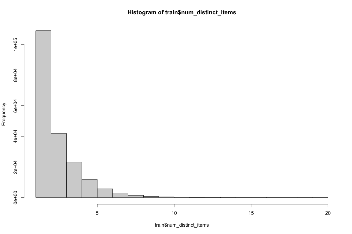
summary(train$num_distinct_items) # no NAs, ranges from 1 to 20
##    Min. 1st Qu.  Median    Mean 3rd Qu.    Max.
##   1.000   1.000   2.000   2.671   3.000  20.000
# looking at the minimum item price
summary(train$min_item_price)  # has negative numbers, like -86, need to exclude it.
##    Min. 1st Qu.  Median    Mean 3rd Qu.    Max.
##   -86.0   299.0   595.0   686.2   949.0 14700.0

train$min_item_price[train$min_item_price < 0] = NA  # after the exclusion, the price for min-price is 0

# looking at the maximum item price
summary(train$max_item_price)  # min is 0
##    Min. 1st Qu.  Median    Mean 3rd Qu.    Max.
##       0     800    1095    1160    1395   14700

## the min and maximum item price are not very
## interpretable or informative. Further, many delivery's
## minimum and maximum item price are overlapping, since
## they just ordered one item. The essential info can be
## captured by subtotal and # of items. They will be
## removed from the models.


# Looking at the supply side of the delivery capacity ---
# on-shift dasher
table(train$total_onshift_dashers)  # has a couple of negative values, will leave them as it is since the train data also has negative values.
##
##   -4   -3   -2   -1    0    1    2    3    4    5    6    7    8    9   10   11
##    1    1   13    6 3615  950 1622 2212 2624 2607 2727 2753 2579 2752 2756 2719
##   12   13   14   15   16   17   18   19   20   21   22   23   24   25   26   27
## 2699 2720 2733 2912 2691 2737 2924 2824 2738 2841 2747 2719 2752 2752 2281 2293
##   28   29   30   31   32   33   34   35   36   37   38   39   40   41   42   43
## 2107 2046 1988 1997 1812 1742 1883 1740 1853 1700 1709 1991 2002 1705 1726 1645
##   44   45   46   47   48   49   50   51   52   53   54   55   56   57   58   59
## 1778 1520 1587 1825 1778 1824 1680 1643 1739 1553 1632 1510 1429 1360 1358 1462
##   60   61   62   63   64   65   66   67   68   69   70   71   72   73   74   75
## 1307 1313 1278 1188 1115 1219  998 1285 1125 1191 1057 1098 1146  934  875  961
##   76   77   78   79   80   81   82   83   84   85   86   87   88   89   90   91
##  863  723  763  762  685  696  696  770  660  636  784  790  733  777  738  708
##   92   93   94   95   96   97   98   99  100  101  102  103  104  105  106  107
##  658  704  591  527  663  799  778  761  678  590  689  687  606  592  537  553
##  108  109  110  111  112  113  114  115  116  117  118  119  120  121  122  123
##  688  453  508  337  335  325  540  366  558  401  382  399  293  242  218  464
##  124  125  126  127  128  129  130  131  132  133  134  135  136  137  138  139
##  352  386  347  397  384  402  383  354  284  282  197  119  203  154  145  106
##  140  141  142  143  144  145  146  147  148  149  150  151  152  153  154  155
##  127  130   20   72  116   95   96   53   96   86   30  113   28   47   21   21
##  156  157  158  159  160  162  163  164  165  168  169  171
##   35   29   19    1    9    1    1    1    1    1    1    1

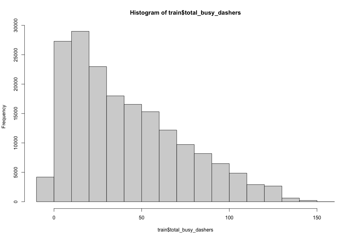
# looking at busy dashers
table(train$total_busy_dashers)  # has a couple of negative values, will leave them as it is since the train data also has negative values.
##
##   -5   -4   -3   -2   -1    0    1    2    3    4    5    6    7    8    9   10
##    1    2    2    3   13 4171 1596 2286 2644 2841 2931 3040 2923 2977 2934 3114
##   11   12   13   14   15   16   17   18   19   20   21   22   23   24   25   26
## 2981 2954 3052 2916 2920 2935 2868 3001 2789 2563 2556 2547 2718 2610 2292 2207
##   27   28   29   30   31   32   33   34   35   36   37   38   39   40   41   42
## 2099 2063 2045 1848 1853 1861 1789 1803 1900 1750 1653 1701 1883 1807 1768 1591
##   43   44   45   46   47   48   49   50   51   52   53   54   55   56   57   58
## 1601 1557 1737 1709 1726 1613 1644 1611 1671 1675 1618 1465 1451 1532 1438 1483
##   59   60   61   62   63   64   65   66   67   68   69   70   71   72   73   74
## 1504 1471 1514 1237 1310 1429 1287 1215 1137 1111 1072  872  998 1120 1156 1115
##   75   76   77   78   79   80   81   82   83   84   85   86   87   88   89   90
##  945  877  876 1033  774  831  877  814  816  786  982  898  859  867  788  504
##   91   92   93   94   95   96   97   98   99  100  101  102  103  104  105  106
##  780  703  679  558  527  571  860  832  524  449  533  553  534  485  351  534
##  107  108  109  110  111  112  113  114  115  116  117  118  119  120  121  122
##  559  474  463  371  253  378  210  382  283  441  201  300  214  254  292  333
##  123  124  125  126  127  128  129  130  131  132  133  134  135  136  137  138
##  335  374  292  246  186  193  261  152  121  112   40   41   48   84   80   64
##  139  140  141  142  143  144  145  146  147  148  149  150  152  153  154
##   23    7   31   45   25    8   36   29    7   31    1    2    2    1    1
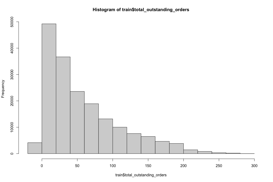
# looking at the outstanding orders, which reduces the
# capacity

table(train$total_outstanding_orders)  # has a couple of negative values, will leave them as it is since the train data also has negative values.
##
##   -6   -5   -4   -3   -2   -1    0    1    2    3    4    5    6    7    8    9
##    5    6    3    8    6   16 4111 1511 2079 2334 2487 2559 2672 2621 2685 2744
##   10   11   12   13   14   15   16   17   18   19   20   21   22   23   24   25
## 2705 2586 2559 2618 2516 2460 2390 2379 2566 2316 2433 2290 2267 2228 2111 2249
##   26   27   28   29   30   31   32   33   34   35   36   37   38   39   40   41
## 2014 1916 1886 1896 1873 1768 1878 1648 1795 1527 1506 1613 1511 1450 1259 1381
##   42   43   44   45   46   47   48   49   50   51   52   53   54   55   56   57
## 1301 1367 1205 1239 1162 1229 1161 1255 1080 1249 1113 1105 1264 1075 1207 1016
##   58   59   60   61   62   63   64   65   66   67   68   69   70   71   72   73
## 1131 1184  864 1072 1133 1085 1077 1106 1050 1018  931  942  875  876  929  952
##   74   75   76   77   78   79   80   81   82   83   84   85   86   87   88   89
##  934  848  918  707  775  908  780  821  702  874  725  671  739  721  699  634
##   90   91   92   93   94   95   96   97   98   99  100  101  102  103  104  105
##  572  694  755  567  618  649  532  695  514  498  489  484  493  553  570  372
##  106  107  108  109  110  111  112  113  114  115  116  117  118  119  120  121
##  559  452  519  495  432  549  574  547  565  477  501  477  515  564  325  520
##  122  123  124  125  126  127  128  129  130  131  132  133  134  135  136  137
##  435  541  363  411  367  525  297  372  407  339  356  257  356  311  453  453
##  138  139  140  141  142  143  144  145  146  147  148  149  150  151  152  153
##  241  307  295  285  438  386  312  409  318  338  365  289  293  300  424  269
##  154  155  156  157  158  159  160  161  162  163  164  165  166  167  168  169
##  395  243  333  324  255  360  165  303  293  304  278  305  203  288  136  248
##  170  171  172  173  174  175  176  177  178  179  180  181  182  183  184  185
##  209  229  211  171  172  204  200  236  230  180  259  243  161  249  161  243
##  186  187  188  189  190  191  192  193  194  195  196  197  198  199  200  201
##  164  122  215  271  221  158  212  215  111  179  159  195  214  182  175  160
##  202  203  204  205  206  207  208  209  210  211  212  213  214  215  216  217
##   86   79   61  161    7   57   90   53  110   57   57   50   73   66   55  120
##  218  219  220  221  222  223  224  225  226  227  228  229  230  231  232  233
##   47   12   37   44   38   69   12   80   70    6   63   36   73  102   43    6
##  234  235  236  237  238  239  240  241  242  243  244  245  246  247  248  249
##   18   18   46   17   30   27   29    3   14   30   13    1   24   19   17   13
##  250  251  252  253  254  256  257  258  259  260  261  262  264  265  268  269
##   24   35   27   45   17   29   11   16    2    1   22   17    1    1    1   21
##  270  272  273  274  276  277  278  283  285
##   19   33    1   14   35    1   20    1    1
# looking at the estimated duration to for the resturant to
# receive an order
order_place_duration_summary = summary(train$estimated_order_place_duration)  # min is 0, max is 2715

# looking at the estimated point-to-point delivery time
store_to_consumer_summary = summary(train$estimated_store_to_consumer_driving_duration)  # has many NA values, min is 0, max is 2088
At this point of pre-processing, it becomes clear that variables like maximum and minimum item prices are neither meaningful nor necessary for predicting delivery time. The subtotal and number of items can capture information about the food ordered that is relevant to the time prediction.
- Based on the existing data, some useful new features like “Weekday or Weekend” and “Day or Night” can be created
train = train %>%
  mutate(actual_duration_sec = as.numeric(actual_delivery_time -created_at)*60,
         # the new variable captures the time that cannot be captured by the point-to-point and order-receive time
         diff_actual_estimate_sec = actual_duration_sec - (estimated_store_to_consumer_driving_duration + estimated_order_place_duration),

          DayOrNight = case_when(
           hour(train$created_at) >= 7 & hour(train$created_at) < 18 ~ "Day",
           TRUE ~ "Night"),

         WeekdayOrWeekend = case_when(
           weekdays(train$created_at) == "Friday" ~ "Weekend",
           weekdays(train$created_at) == "Saturday" ~ "Weekend",
           weekdays(train$created_at) == "Sunday" ~ "Weekend",
           TRUE ~ "Weekday")

    )


test = test %>%
  mutate( DayOrNight = case_when(
           hour(test$created_at) >= 7 & hour(test$created_at) < 18 ~ "Day",
           TRUE ~ "Night"),

         WeekdayOrWeekend = case_when(
           weekdays(test$created_at) == "Friday" ~ "Weekend",
           weekdays(test$created_at) == "Saturday" ~ "Weekend",
           weekdays(test$created_at) == "Sunday" ~ "Weekend",
           TRUE ~ "Weekday")

    )
- Since I decided to not include uninformative variables like maximum item price when predicting, I’ll only select relevant columns to be included in the cleaned train and raw dataset.
selected_data = as.data.frame(train[, c(1, 4:8, 12:16, 18:20)])


selected_data_test = as.data.frame(test[, c(1, 3:7, 11:15, 18,
    19, 16)])
Selecting metrics
I’d evaluate the models based on the aspect that matters to the business goal the most. Since severe underestimation of delivery time (i.e., being late over 10 minutes) would be really painful for the customers, the model that better reduce the late over 10 minute would be better. Further, the penalization of being late, even within 5 minutes, should be more than the being early when comparing the existing and the potential new model.
-
The first model is a linear regression model with all the variables left after feature engineering as predictors. The second model is a linear mixed effect model with store_id as a random effect (since we are not intestered in the clustering effect introduced by each specific stores).
-
The linear regression model and the mixed effect model outcomes were compared based on their Root Mean Square Error (RMSE) and their percentage of underestimating the delivery time (being late is bad).
-
The mixed effect model outperforms the linear regression model in both RMSE and the reduced overall lateness (14.93% -> 14.1%) and reduced significant-late (6.9% -> 6.3%). The predicted values from the mixed effect model will be keep to compare with the next model.
set.seed(100)
TrainingIndex <- createDataPartition(selected_data$diff_actual_estimate_sec[!is.na(selected_data$diff_actual_estimate_sec)],
    p = 0.8, list = FALSE)
TrainingSet <- selected_data[TrainingIndex, ]  # Training Set
TestingSet <- selected_data[-TrainingIndex, ]  # Test Set

# below is a linear regression model with store_id removed,
# further, the primary store category of a store is also
# removed since new categories were added to the testing
# dataset the code below shows that there are new store
# categories
train_category = as.data.frame(table(selected_data$store_primary_category))$Var1
test_category = as.data.frame(table(selected_data_test$store_primary_category))$Var1
new_categoryInTesting = unique(train_category[!train_category %in%
    test_category])  #belgian   chocolate lebanese
old_categoryOnlyInTraining = unique(test_category[!test_category %in%
    train_category])  # non of them are new to the test dataset but old to the train dataset

lm_model <- lm(diff_actual_estimate_sec ~ market_id + order_protocol +
    total_items + subtotal + total_onshift_dashers + total_busy_dashers +
    total_outstanding_orders + DayOrNight + WeekdayOrWeekend +
    estimated_order_place_duration + estimated_store_to_consumer_driving_duration,
    data = TrainingSet)


#### rsme for lm model formula from
#### https://stackoverflow.com/questions/43123462/how-to-obtain-rmse-out-of-lm-result
RSS <- c(crossprod(lm_model$residuals))
MSE <- RSS/length(lm_model$residuals)  # faster than mean()
RMSE <- sqrt(MSE)  ##  1026.231

predicted_lm <- predict(lm_model, newdata = TestingSet)


lm_error = TestingSet$diff_actual_estimate_sec - (predicted_lm +
    TestingSet$estimated_order_place_duration + TestingSet$estimated_store_to_consumer_driving_duration)
ErrorEvaluation_lm = data.frame(lm_error = lm_error, EarlyLateCategory = case_when(lm_error >
    10 * 60 ~ "Late Over 10 Min", lm_error <= 10 * 60 & lm_error >
    5 * 60 ~ "Late 5-10 Min", lm_error <= 5 * 60 & lm_error >
    0 ~ "Late within 5 Min", lm_error <= 0 & lm_error > -5 *
    60 ~ "Early within 5 Min", lm_error <= -5 * 60 & lm_error >
    -10 * 60 ~ "Early 5-10 Min", lm_error <= -10 * 60 ~ "Early more than 10 Min"))
## looking at the distribution of the early and late
## category, there are currently

ErrorEvaluation_lm_EarlyLateCategory = as.data.frame(prop.table(table(ErrorEvaluation_lm$EarlyLateCategory)))

colnames(ErrorEvaluation_lm_EarlyLateCategory) = c("Early Late Category",
    "Frequency")

level_category <- c("Early more than 10 Min", "Early 5-10 Min",
    "Early within 5 Min", "Late within 5 Min", "Late 5-10 Min",
    "Late Over 10 Min")

ErrorEvaluation_lm_EarlyLateCategory = ErrorEvaluation_lm_EarlyLateCategory %>%
    mutate(`Early Late Category` = factor(`Early Late Category`,
        levels = level_category)) %>%
    arrange(`Early Late Category`)

table_ErrorEvaluation_lm_EarlyLateCategory = ErrorEvaluation_lm_EarlyLateCategory %>%
    knitr::kable(digits = 3, caption = "Error Evaluation Linear Regression Model Early Late Category") %>%
    kableExtra::kable_styling(latex_options = "scale_down")


# the simple linear model also does well in having an
# overall lateness of 14.93%. But its very late category
# (6.9%) is higher than the mixed effect model prediction
# (below)

TrainingSet$market_id[is.na(TrainingSet$market_id) == T] = "NA"
TrainingSet$order_protocol[is.na(TrainingSet$order_protocol) ==
    T] = "NA"
lmer_model <- lmer(diff_actual_estimate_sec ~ market_id + order_protocol +
    total_items + subtotal + total_onshift_dashers + total_busy_dashers +
    total_outstanding_orders + estimated_order_place_duration +
    estimated_store_to_consumer_driving_duration + DayOrNight +
    WeekdayOrWeekend + (1 | store_id), data = TrainingSet)

lmer_rmse = RMSE.merMod(lmer_model)  #  958.1015

TestingSet$market_id[is.na(TestingSet$market_id) == T] = "NA"
TestingSet$order_protocol[is.na(TestingSet$order_protocol) ==
    T] = "NA"

newdata = TestingSet %>%
    dplyr::select(diff_actual_estimate_sec, market_id, order_protocol,
        total_items, subtotal, total_onshift_dashers, total_busy_dashers,
        total_outstanding_orders, estimated_order_place_duration,
        estimated_store_to_consumer_driving_duration, DayOrNight,
        WeekdayOrWeekend, store_id)

predicted_lmer <- predict(lmer_model, newdata = newdata, allow.new.levels = TRUE)

lmer_error = TestingSet$diff_actual_estimate_sec - (predicted_lmer +
    TestingSet$estimated_order_place_duration + TestingSet$estimated_store_to_consumer_driving_duration)
ErrorEvaluation_lmer = data.frame(lmer_error = lmer_error, EarlyLateCategory = case_when(lmer_error >
    10 * 60 ~ "Late Over 10 Min", lmer_error <= 10 * 60 & lmer_error >
    5 * 60 ~ "Late 5-10 Min", lmer_error <= 5 * 60 & lmer_error >
    0 ~ "Late within 5 Min", lmer_error <= 0 & lmer_error > -5 *
    60 ~ "Early within 5 Min", lmer_error <= -5 * 60 & lmer_error >
    -10 * 60 ~ "Early 5-10 Min", lmer_error <= -10 * 60 ~ "Early more than 10 Min"))
lmer_summary = prop.table(table(ErrorEvaluation_lmer$EarlyLateCategory))

# The vast majority of the delivery is early under this
# model, the overall lateness is 14.1%. The the very (over
# 10 min) late category is around 6.3% percent


ErrorEvaluation_lmixed_EarlyLateCategory = as.data.frame(prop.table(table(ErrorEvaluation_lmer$EarlyLateCategory)))

colnames(ErrorEvaluation_lmixed_EarlyLateCategory) = c("Early Late Category",
    "Frequency")

level_category <- c("Early more than 10 Min", "Early 5-10 Min",
    "Early within 5 Min", "Late within 5 Min", "Late 5-10 Min",
    "Late Over 10 Min")


ErrorEvaluation_lmixed_EarlyLateCategory = ErrorEvaluation_lmixed_EarlyLateCategory %>%
    mutate(`Early Late Category` = factor(`Early Late Category`,
        levels = level_category)) %>%
    arrange(`Early Late Category`)

table_ErrorEvaluation_lmixed_EarlyLateCategory = ErrorEvaluation_lmixed_EarlyLateCategory %>%
    knitr::kable(digits = 3, caption = "Error Evaluation Linear MIXED Model Early Late Category") %>%
    kableExtra::kable_styling(latex_options = "scale_down")
| Early Late Category | Frequency |
|---|---|
| Early more than 10 Min | 0.677 |
| Early 5-10 Min | 0.102 |
| Early within 5 Min | 0.072 |
| Late within 5 Min | 0.050 |
| Late 5-10 Min | 0.031 |
| Late Over 10 Min | 0.069 |
| Early Late Category | Frequency |
|---|---|
| Early more than 10 Min | 0.682 |
| Early 5-10 Min | 0.105 |
| Early within 5 Min | 0.073 |
| Late within 5 Min | 0.048 |
| Late 5-10 Min | 0.030 |
| Late Over 10 Min | 0.063 |
- The third prediction model for consideration is a XGBoost model
First, I used one-hot encoding to ensure that training is a numeric metric before the XGBoost modeling.
# one_hot_encoding

TrainingSet = TrainingSet %>%
    filter(market_id != "NA")

TrainingSet = TrainingSet %>%
    filter(order_protocol != "NA")

dummy <- dummyVars(" ~ .", data = as.data.frame(TrainingSet[,
    c(1, 4, 13, 14)]))

newdata <- data.frame(predict(dummy, newdata = as.data.frame(TrainingSet[,
    c(1, 4, 13, 14)])))

newdata[is.na(newdata)] = 0


# imputing the missing values for the xgboost
RestOfOneHotEncoded = as.data.frame(TrainingSet[, -c(1:4, 13,
    14)])
RestOfOneHotEncoded$diff_actual_estimate_sec[is.na(RestOfOneHotEncoded$diff_actual_estimate_sec)] <- median(RestOfOneHotEncoded$diff_actual_estimate_sec,
    na.rm = TRUE)
RestOfOneHotEncoded$estimated_store_to_consumer_driving_duration[is.na(RestOfOneHotEncoded$estimated_store_to_consumer_driving_duration)] <- median(RestOfOneHotEncoded$estimated_store_to_consumer_driving_duration,
    na.rm = TRUE)
RestOfOneHotEncoded$total_outstanding_orders[is.na(RestOfOneHotEncoded$total_outstanding_orders)] <- median(RestOfOneHotEncoded$total_outstanding_orders,
    na.rm = TRUE)
RestOfOneHotEncoded$total_onshift_dashers[is.na(RestOfOneHotEncoded$total_onshift_dashers)] <- median(RestOfOneHotEncoded$total_onshift_dashers,
    na.rm = TRUE)
RestOfOneHotEncoded$total_busy_dashers[is.na(RestOfOneHotEncoded$total_busy_dashers)] <- median(RestOfOneHotEncoded$total_busy_dashers,
    na.rm = TRUE)

OneHotEncoded = cbind(newdata, RestOfOneHotEncoded)
TestingSet = TestingSet %>%
    filter(market_id != "NA")

TestingSet = TestingSet %>%
    filter(order_protocol != "NA")

# one_hot_encoding
dummy_test <- dummyVars(" ~ .", data = as.data.frame(TestingSet[,
    c(1, 4, 13, 14)]))

newdata_test <- data.frame(predict(dummy_test, newdata = as.data.frame(TestingSet[,
    c(1, 4, 13, 14)])))
newdata_test[is.na(newdata_test)] = 0

# imputing the missing values for the xgboost
RestOfOneHotEncoded_test = as.data.frame(TestingSet[, -c(1:4,
    13, 14)])
RestOfOneHotEncoded_test$estimated_store_to_consumer_driving_duration[is.na(RestOfOneHotEncoded_test$estimated_store_to_consumer_driving_duration)] <- median(RestOfOneHotEncoded_test$estimated_store_to_consumer_driving_duration,
    na.rm = TRUE)
RestOfOneHotEncoded_test$total_outstanding_orders[is.na(RestOfOneHotEncoded_test$total_outstanding_orders)] <- median(RestOfOneHotEncoded_test$total_outstanding_orders,
    na.rm = TRUE)
RestOfOneHotEncoded_test$total_onshift_dashers[is.na(RestOfOneHotEncoded_test$total_onshift_dashers)] <- median(RestOfOneHotEncoded_test$total_onshift_dashers,
    na.rm = TRUE)
RestOfOneHotEncoded_test$total_busy_dashers[is.na(RestOfOneHotEncoded_test$total_busy_dashers)] <- median(RestOfOneHotEncoded_test$total_busy_dashers,
    na.rm = TRUE)

OneHotEncoded_test = cbind(newdata_test, RestOfOneHotEncoded_test)
# put our testing & training data into two seperates
# Dmatrixs objects
dtrain <- xgb.DMatrix(data = as.matrix(OneHotEncoded[, colnames(OneHotEncoded) !=
    "diff_actual_estimate_sec"]), label = OneHotEncoded$diff_actual_estimate_sec)
dtest <- xgb.DMatrix(data = as.matrix(OneHotEncoded_test[, colnames(OneHotEncoded_test) !=
    "diff_actual_estimate_sec"]))
In addition, I am taking over the best tuned values from the caret cross validation.
#### parameters inspired by https://www.kaggle.com/erikbruin/house-prices-lasso-xgboost-and-a-detailed-eda/report
default_param<-list(
        objective = "reg:squarederror",
        booster = "gbtree",
        eta=0.03,
        gamma=0,
        max_depth=3, #default=6
        min_child_weight=1, #default=1
        subsample=1,
        colsample_bytree=1
)
The next step is cross validate to determine the best number of rounds (for the given set of parameters).
set.seed(100)
xgbcv <- xgb.cv(params = default_param, data = dtrain, nrounds = 500,
    nfold = 7, showsd = T, stratified = T, print_every_n = 50,
    early_stopping_rounds = 10, maximize = F)
## [1]  train-rmse:2581.498929+82.965879    test-rmse:2542.178573+456.683671
## Multiple eval metrics are present. Will use test_rmse for early stopping.
## Will train until test_rmse hasn't improved in 10 rounds.
##
## [51] train-rmse:1690.397292+126.490097   test-rmse:1584.052969+656.953643
## [101]    train-rmse:1600.839812+126.288823   test-rmse:1509.279747+678.493756
## [151]    train-rmse:1581.010156+124.756873   test-rmse:1498.199457+680.784268
## [201]    train-rmse:1565.436911+124.052633   test-rmse:1492.758189+682.300756
## [251]    train-rmse:1551.546785+122.809176   test-rmse:1488.235455+684.318066
## [301]    train-rmse:1542.022058+121.625511   test-rmse:1485.011633+685.894950
## [351]    train-rmse:1534.317781+121.241970   test-rmse:1482.886396+687.301957
## Stopping. Best iteration:
## [373]    train-rmse:1531.970765+120.833297   test-rmse:1481.976564+687.507665
# [1]\ttrain-rmse:2248.431566+4.564152\ttest-rmse:2248.275217+27.603266
# Multiple eval metrics are present. Will use test_rmse for
# early stopping.  Will train until test_rmse hasn't
# improved in 10 rounds.
# [51]\ttrain-rmse:1155.453953+6.996119\ttest-rmse:1155.530700+44.531763
# [101]\ttrain-rmse:1058.757189+7.407113\ttest-rmse:1059.669081+46.052753
# [151]\ttrain-rmse:1040.796808+7.226292\ttest-rmse:1042.572885+46.117138
# [201]\ttrain-rmse:1029.334863+7.374779\ttest-rmse:1031.947599+45.965339
# [251]\ttrain-rmse:1020.872993+7.404225\ttest-rmse:1024.585417+45.954483
# [301]\ttrain-rmse:1014.524255+7.407507\ttest-rmse:1019.136701+46.050757
# [351]\ttrain-rmse:1009.616736+7.337194\ttest-rmse:1015.069901+46.052787
# [401]\ttrain-rmse:1005.703525+7.237976\ttest-rmse:1012.005312+46.090358
# [451]\ttrain-rmse:1002.528861+7.204019\ttest-rmse:1009.440472+46.026105
# [500]\ttrain-rmse:1000.040400+7.151973\ttest-rmse:1007.622563+46.082395
# train the model using the best iteration found by cross
# validation
xgb_mod <- xgb.train(data = dtrain, params = default_param, nrounds = 442)
XGBpred <- predict(xgb_mod, dtest)
After obtaining the RMSE score, I use the pre-constructed early/late category to evaluate the XGBoost model. As presented below, the result shows that this model is by large overestimating the delivery time, which is less evil than underestimating the delivery time. However, its percentage of being very (over 10 min) early ranks between the linear regression and the linear mixed effect model.
xgboost_error = TestingSet$diff_actual_estimate_sec - (round(XGBpred) +
    TestingSet$estimated_order_place_duration + TestingSet$estimated_store_to_consumer_driving_duration)
xgboostErrorEvaluation = data.frame(xgboost_error = xgboost_error,
    EarlyLateCategory = case_when(xgboost_error > 10 * 60 ~ "Late Over 10 Min",
        xgboost_error <= 10 * 60 & xgboost_error > 5 * 60 ~ "Late 5-10 Min",
        xgboost_error <= 5 * 60 & xgboost_error > 0 ~ "Late within 5 Min",
        xgboost_error <= 0 & xgboost_error > -5 * 60 ~ "Early within 5 Min",
        xgboost_error <= -5 * 60 & xgboost_error > -10 * 60 ~
            "Early 5-10 Min", xgboost_error <= -10 * 60 ~ "Early more than 10 Min"))
## looking at the distribution of the early and late
## category, there are currently
prop.table(table(xgboostErrorEvaluation$EarlyLateCategory))
##
##         Early 5-10 Min Early more than 10 Min     Early within 5 Min
##             0.09872233             0.68068311             0.07235927
##          Late 5-10 Min       Late Over 10 Min      Late within 5 Min
##             0.03208096             0.06783049             0.04832385
# this result indicates the XGBoost model has significantly
# lower RMSE, but higher 'late over 10 min' percentage. The
# overall lateness of the XGBoost (14.9%) is similar with
# the rest of the two models

# Early 5-10 Min Early more than 10 Min 0.10099015
# 0.68001216 Early within 5 Min Late 5-10 Min 0.07202006
# 0.03327509 Late Over 10 Min Late within 5 Min 0.06738585
# 0.04631670

ErrorEvaluation_xgboost_EarlyLateCategory = as.data.frame(prop.table(table(xgboostErrorEvaluation$EarlyLateCategory)))

colnames(ErrorEvaluation_xgboost_EarlyLateCategory) = c("Early Late Category",
    "Frequency")

level_category <- c("Early more than 10 Min", "Early 5-10 Min",
    "Early within 5 Min", "Late within 5 Min", "Late 5-10 Min",
    "Late Over 10 Min")

ErrorEvaluation_xgboost_EarlyLateCategory = ErrorEvaluation_xgboost_EarlyLateCategory %>%
    mutate(`Early Late Category` = factor(`Early Late Category`,
        levels = level_category)) %>%
    arrange(`Early Late Category`)

table_ErrorEvaluation_xgboost_EarlyLateCategory = ErrorEvaluation_xgboost_EarlyLateCategory %>%
    knitr::kable(digits = 3, caption = "Error Evaluation XGBoost Model Early Late Category") %>%
    kableExtra::kable_styling(latex_options = "scale_down")
| Early Late Category | Frequency |
|---|---|
| Early more than 10 Min | 0.681 |
| Early 5-10 Min | 0.099 |
| Early within 5 Min | 0.072 |
| Late within 5 Min | 0.048 |
| Late 5-10 Min | 0.032 |
| Late Over 10 Min | 0.068 |
- By evaluating the RMSE and lateness category of the XGBoost model, I found out that the XGBoost’s RMSE score is much better than the linear regression and mixed effect models. However, the mixed effect model has lower “very late” delivery than the XGBoost model. Thus, in the submission, I average the XGBoost and the mixed effect model prediction, with a heavier weight given to the XGBoost model.
# one_hot_encoding for submission data
dummy_submit <- dummyVars(" ~ .", data = as.data.frame(test[,
    c(1, 5, 18, 19)]))  # the platform feature is new. I omit it since it's absent in the training data

newdata_submit <- data.frame(predict(dummy_submit, newdata = as.data.frame(test[,
    c(1, 5, 18, 19)])))
newdata_submit[is.na(newdata_submit)] = 0

# imputing the missing values for the xgboost
RestOfOneHotEncoded_submit = as.data.frame(test[, -c(1:5, 8:10,
    16:19)])
RestOfOneHotEncoded_submit$estimated_store_to_consumer_driving_duration[is.na(RestOfOneHotEncoded_submit$estimated_store_to_consumer_driving_duration)] <- median(RestOfOneHotEncoded_submit$estimated_store_to_consumer_driving_duration,
    na.rm = TRUE)
RestOfOneHotEncoded_submit$total_outstanding_orders[is.na(RestOfOneHotEncoded_submit$total_outstanding_orders)] <- median(RestOfOneHotEncoded_submit$total_outstanding_orders,
    na.rm = TRUE)
RestOfOneHotEncoded_submit$total_onshift_dashers[is.na(RestOfOneHotEncoded_submit$total_onshift_dashers)] <- median(RestOfOneHotEncoded_submit$total_onshift_dashers,
    na.rm = TRUE)
RestOfOneHotEncoded_submit$total_busy_dashers[is.na(RestOfOneHotEncoded_submit$total_busy_dashers)] <- median(RestOfOneHotEncoded_submit$total_busy_dashers,
    na.rm = TRUE)

OneHotEncoded_submit = cbind(newdata_submit, RestOfOneHotEncoded_submit)

dsubmit <- xgb.DMatrix(data = as.matrix(OneHotEncoded_submit))

XGB_pred_submmit <- predict(xgb_mod, dsubmit)


test$market_id[is.na(test$market_id) == T] = "NA"
test$order_protocol[is.na(test$order_protocol) == T] = "NA"

sub_avg <- data.frame(delivery_id = test$delivery_id, `predicted duration` = (2 *
    XGB_pred_submmit + predict(lmer_model, newdata = test, allow.new.levels = TRUE))/3)


write.csv(sub_avg, "final_output.csv",
    row.names = F)